Continuity, Jumps, and Measuring Progress

Up until now, we’ve discussed a framework for potential here, explored the nature of the game we want to play here, and examined one possible model to go from point A to point B here. In this article, I’ll delve into the very act of measuring progress, defined as movement from point A to point B. I believe progress should be viewed as a combination of (i) continuous improvement and (ii) jumps. While the former helps us stay in the game, the latter leads to exponential gains and provides milestones to mark the passage of time, offering incentives to keep pursuing our goals, especially when the continuous nature of the former attribute becomes repetitive and/or mundane and might lead to giving up the pursuit altogether.
Before we proceed any further with this investigation, it is quite important to understand the implications of progress as a function of a continuous process and jumps on the passage of time.
Model
In almost all modern conceptualisations, time is taken to be “continuous,” meaning it is infinitely divisible as far as the mind can comprehend. From an observational standpoint, I often struggle with continuity as a concept, probably due to cognitive limitations in measuring things continuously on an infinitely divisible timescale. In fact, I believe that for the most part, we don’t even track the “passage of time” continuously. It seems more likely that we become “aware” of the passage of time at randomly spaced intervals. In such moments, while we still don’t feel time “passing by,” we certainly become aware of time “passed by” since our last such realisation. As such, I believe that at randomly spaced intervals we experience a “jump” event that makes us conscious of the fact that time has “passed by”.
To explore this further, let’s clarify the distinction between measuring time and feeling the passage of time. For our purposes, we are more interested in the latter, as I believe that psychologically it is more pertinent to understanding our behaviour in the context of pursuing tasks and measuring progress.
Let’s engage in a thought experiment. Imagine you are in a sensory deprivation tank that eliminates all external stimuli such as light, sound, and tactile sensations. Further, assume that you have not been introduced to the concept of counting and have no conception of a clock. In this sensory deprivation tank, you have a peephole that allows you to observe the outside world. Your perception of the passage of “time,” insofar as you can even conceptualise a thing called “time”, will likely be determined by your observations through the peephole. More specifically, your experience of the passage of time will depend on the movement within the observed landscape through the peephole. The more movement occurs within the landscape, the more you’ll observe, and the more you’ll register as events “happening”.
Your observation of what the landscape was versus what it currently is would probably be the best possible method of noting that reality is in motion. In other words, if the landscape you observe through the peephole reflects a singular, non-fluctuating event, there would be no way for you to confirm if reality is at a standstill or not, thus making the passage of time impossible to verify. As such, we can say that in this experiment it is the rate of change in the composition of the landscape that you observe that helps you become aware of reality and, consequently, of reality being in motion.
Before we move on to the implications of this model, let us already recap what we have discussed so far.
-
We discussed progress, i.e., moving forward from point A to point B, as a combination of continuous movement and something called “jumps”.
-
We examined our understanding of the passage of time. We noted that, for the most part, it seems we don’t continuously track time but only become aware of its passage due to a “jump” that we experience at randomly spaced intervals.
-
We conducted a thought experiment where we concluded that in instances where we receive extremely limited information, our understanding of the passage of time is restricted to the rate of change of the information we receive.
Implications
Now, in practice, when moving from point A to point B, we chart a territory for ourselves. In the deepest sense of pursuing something of higher value, it’s not far-fetched to assume that this is a meaningful pursuit. We can then assume that when we are in this pursuit, we are solely focused on it, blocking out any possible distractions, akin to being in a sensory deprivation tank where we have a peephole through which we can see point B and nothing else.
Initially, as we move towards point B, we are in an excited state due to the novelty of the task and are quite aware of movement(s) or time “passing by.” However, as we continue moving forward, the continuous nature of the path becomes mundane from a sensory perspective. In the context of the thought experiment, through the peephole, we see point B slowly coming closer, but only marginally so. As a result, the rate of change in the landscape reduces, making us unaware of the passage of time.
It is only when a jump event occurs that we once again become aware of the passage of time, allowing us to become conscious of our pursuit, reorient ourselves, or correct our path. This is why, although we are often encouraged to believe in incremental, continuous progress that “must” be taking place in this continuous state space, it is difficult for most of us to observe and believe in this progress in practice.
From an experiential standpoint, while we live continuously, we are only able to observe jumps as real markers of the true passage of time and progress.
I suppose that anecdotally, this is the equivalent of us usually saying things like “it feels like time is passing by very slowly” when we are pursuing tasks that seem mundane or tasks that don’t warrant any significant input from ourselves, while when we remark, “i cannot believe how how time flew” are typically for instances where we are highly involved in engaging with the landscape around us.
I cannot underscore the dual nature of mundanity of continuous tasks and the significance of jumps in our pursuit of point B enough. The process of moving from point A to point B often involves repeating the same types of tasks, much like the gradient ascent algorithm we explored in the previous article. It is natural for us to become accustomed to these tasks. In other words, we may become so familiar with what’s happening around us that we stop actively engaging with the task at hand.
As a consequence of what we’ve discussed, this means that after enough repetitions, we may find it quite hard to engage actively, and thus fail to perceive the passage of time. This is dangerous in our pursuit of progress for two reasons:
-
Misjudgment of Time: If we fail to perceive the flow of time, we may think that we have more time than we realistically do.
-
Loss of Motivation: If we fail to perceive the flow of time and, as a result, lose the ability to mark progress, we may feel stuck in a limbo for too long. This can ultimately lead us to abandon the pursuit of reaching point B altogether.
While the tone may initially appear somewhat somber, there exists a notable silver lining within the concept of “jumps,” which emerges from a standpoint rooted more in observation than theory. Although diving into the origins of such jumps may necessitate dedicated inquiry, I feel that the associated experiential reality is widely acknowledged. Consider the context of running: while continuous progress manifests as incremental timing enhancements, a “jump” can be exemplified by the phenomenon of the “runner’s high.” This euphoric state during a run can lead to significant alterations, enabling runners to either shorten their time or extend their distance considerably. Some runners may even argue that it is these jumps, rather than gradual advancements, that they ultimately seek to attain.
To visualise the concepts we’ve discussed, we’ll need a couple of key ingredients:
-
A continuous time process to represent our progress and,
-
A jump process that we can adjust to see how it affects our progress over time. Thankfully, we don’t have to look too far for these ingredients.
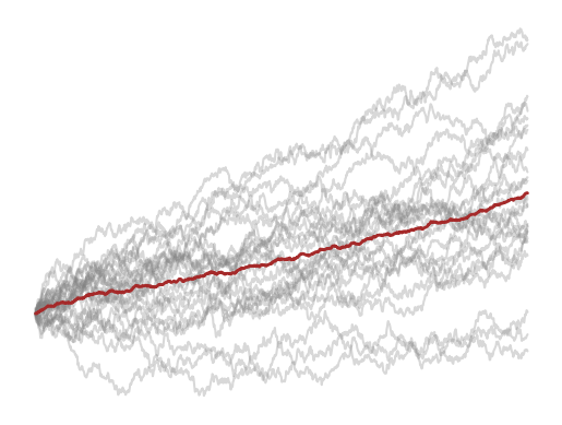
For (1), we’ll use something called a standard Brownian motion with a positive drift to account for some form of upward movement on average. It’s a fancy way of saying it’s a smooth, random process that’s great for modelling things where changes happen continuously and unpredictably. Brownian motion is really versatile and gets used in lots of different fields, like finance, physics, and biology.
# Define the number of steps, the step size, and the number of paths
num_steps = 1000
step_size = 1
mu = 50
num_paths = 25

# Initialize an array to store the paths
paths = np.zeros((num_paths, num_steps))

# Generate the paths
for i in range(num_paths):
    increments = np.random.normal(loc=mu/num_steps, scale=np.sqrt(step_size), size=num_steps)
    paths[i] = np.cumsum(increments)

# Calculate the mean path
mean_path = np.mean(paths, axis=0)

To model our jumps, we’ll break the problem down into two parts that we’ll add to our standard Brownian motion to create what is known as a Jump Diffusion Process. We’ll define two additional processes: (i) one to represent when jumps happen and (ii) another to represent how big those jumps are when they do occur.
A Poisson process is very well suited to model the arrival of jumps. The Poisson process models the occurrence of discrete events over time.
-
Each event represents a sudden, instantaneous jump, which aligns well with the framework so far.
-
In this case, the number of events occurring in disjoint time intervals are independent. This property ensures that the jumps in our process occur randomly and independently over time.
-
The probability distribution of the number of events in a given time interval depends only on the length of the interval, not on its position. This means that the process is homogeneous over time, which simplifies the modelling of jumps.
As seen in the visualisation below, a Poisson process is defined by a single parameter, lambda. For any lambda greater than 0, this process won’t have a mean of 0. So, for our visualisation purposes, we need to tweak this process slightly. We do this by creating what’s called a compensated Poisson process. Essentially, we subtract the expected linear growth (lambda times t) from the Poisson process. This adjustment centres the process around zero, effectively making it a martingale. In other words, this allows us to model jumps with a mean zero and allows for the possibility of both, up and down, jumps.

Poisson Distribution: lambda = 3
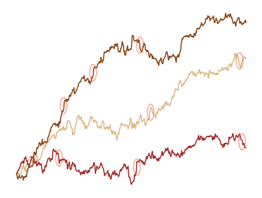
Lastly, we’ll model the intensity of the jumps to follow a normal distribution. With all these components in place, we now have everything we need to model a jump diffusion process. Below is the visual representation of the jump diffusion process. [Author’s note: For this, I am grateful to the wonderful lecture series on Computational Finance by Lech Grzelak that you can find here. I am also grateful for his code repository that I have used for illustrative purposes and noted as such. This can be found here.]

Simulations = 3
Note how, in comparison to the Standard Brownian Motion, the Jump Diffusion process now displays discernible jumps (highlighted in red) and aligns more closely with our proposed framework.
In conclusion, we have now taken another step towards the measuring progress, defined as movement from point A to point B. In exploring the dynamic interplay between continuous improvement and “jumps”, we dived into the intriguing concept of time perception, noting that we don’t consistently track time but rather become aware of its passage through sporadic “jump” events and why this is relevant for measurement of progress towards a goal.
As always, I trust that you found this enriching and thought-provoking. For those inclined to delve deeper into the subject matter, you can find the underlying Python script on GitHub.